Billing data and its limits

Cost governance on Google Cloud generally begins with the detailed usage export, the BigQuery dataset most organizations still refer to as the CUR. The export is authoritative on expenditure. It is not a record of architecture.

A load balancing entry in that export resolves to a service, an SKU, a project, a region, a usage quantity, and a charge: a forwarding rule charge, 730 hours, and a modest dollar amount. Aggregated across an organization, the result is precise to the cent and insufficient to support a remediation decision.

The export does not identify which load balancer the charge belongs to, which of the twelve documented types it represents, whether that type remains appropriate to the traffic it now carries, whether it served any request during the reporting period, when its certificate expires, whether its backends are passing health checks, or whether it is provisioned with more forwarding rules than the billed bundle covers.

None of those attributes is derivable from billing data. Each must be read from the resources themselves and from the telemetry those resources emit. This article describes that process: a single read-only service account scoped to an organisation, a traversal of every load balancer within it, the collection of configuration and metric data for each, the derivation of cost from both, and the generation of recommendations from the combined result.

In Google Cloud load balancing, the billed object and the architectural object are not the same object. A billing line corresponds to a forwarding rule or a volume of processed data, not to the load balancer an engineer would name.

A load balancer is a composite resource

A load balancer named in the Google Cloud console has no corresponding single API resource. The construct is assembled from a set of Compute Engine objects that operate collectively.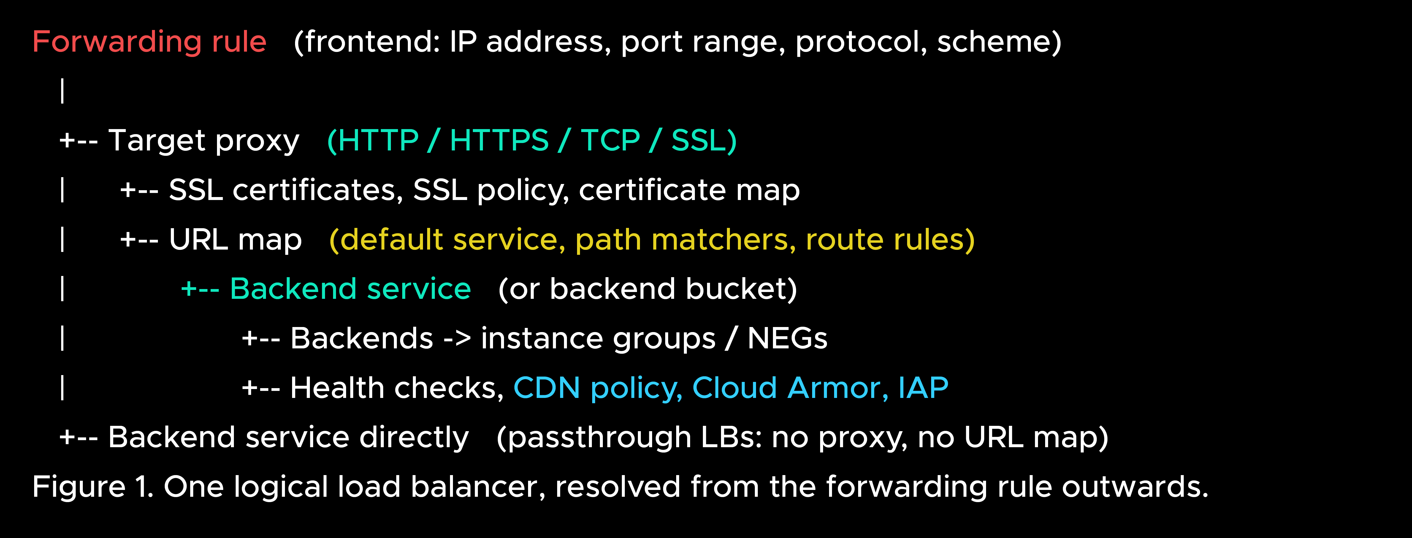

Passthrough network load balancers do not follow the upper path. They have no target proxy and no URL map; the forwarding rule references a backend service directly, or, in the legacy form, a target pool. That structural property, a backend service with no target, is the most reliable classification signal available for the family.

Inventory collection is therefore a graph traversal rather than a list operation. The traversal begins at the forwarding rules, the only resources present for every type without exception, and resolves each outwards: the target it references, the URL map that target uses, the backend services that URL map routes to, the instance groups or network endpoint groups behind those services, and the health checks and policies attached to them. Multiple forwarding rules commonly belong to one logical load balancer, since a frontend serving both IPv4 and IPv6, or both port 80 and port 443, consists of two or three rules and a single load balancer. Consolidating them into one record allows an inventory row to correspond to the entity an engineer recognises and prevents an estate from being reported at several times its actual size.

A second requirement follows from console parity. Not every forwarding rule belongs to a load balancer. Private Service Connect endpoints, Cloud VPN gateways and Cloud Service Each mesh configuration creates forwarding rules, and none of them is listed on the console's load balancing page. Their inclusion produces an inventory that disagrees with the console, which shifts the first review from findings to reconciliation.

The four APIs and the data they contribute

Collection runs under a single service account with read-only access at the audit scope, whether an organisation, a folder or an explicit project list. The roles being: roles/compute.viewer and roles/monitoring.viewer are sufficient, with roles/serviceusage.serviceUsageViewer as an optional addition; roles/compute.networkViewer is not sufficient despite its name, since it does not permit listing instance groups or SSL policies. Nothing is deployed into the audited projects, and no configuration is written back. What follows concerns the data each API contributes and the findings that data supports.

Cloud Resource Manager returns the audit population: every active project beneath the selected scope, with its identifier and project number. The project number is more than an address, since certain Cloud Monitoring resources report load balancer identity with it prefixed to the name. Establishing the population at organizational level is what makes estate-wide findings expressible: backend services referenced from more than one project, duplicated frontends built by separate teams, and idle counts stated as a proportion of the estate rather than of a single project.

Service Usage returns the set of enabled services per project. Its contribution is interpretive rather than descriptive: it distinguishes a project that contains no load balancers from a project on which the Compute Engine API is disabled. The two are identical in the output and entirely different in meaning.

Compute Engine supplies the configuration graph in thirteen list operations per project spanning forwarding rules, target proxies of all four kinds, target pools and target instances, URL maps, backend services and buckets, instance groups and network endpoint groups, and SSL certificates and policies. A further call per backend group returns live health. This is the largest contribution by volume and by finding count.

Cloud Monitoring supplies the behavioral series: request counts split by response code class, request and response bytes, ingress and egress bytes and packets, latency and round-trip time distributions, and connection counts. These are the only values describing what a load balancer has actually done, and they convert a configuration audit into a cost and utilization assessment.

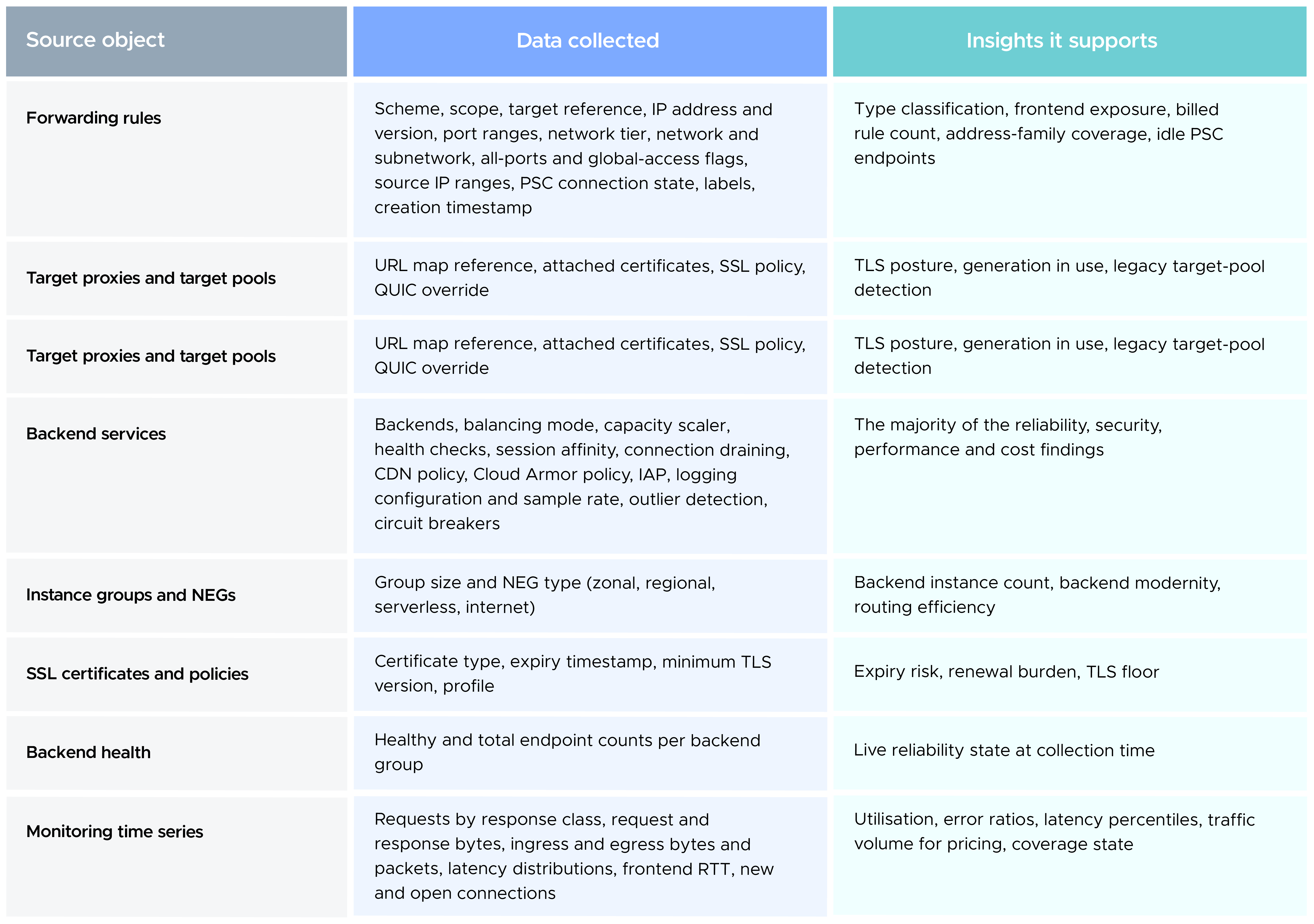
Analysis proceeds in three stages. Collected fields are first normalized into per-load-balancer attributes so that several forwarding rules, proxies and backend services resolve to a single row. Derived values are then computed from combinations of those attributes: certificate expiry in days, error ratios from response-class counts against total requests, data processed from summed ingress and egress, and proxy instance counts from sustained throughput. Findings are finally evaluated as threshold and presence tests across the combined set, which allows one finding to depend on configuration and telemetry simultaneously. A recommendation to remove an idle load balancer requires a measured request count of zero, a coverage state confirming the measurement was taken, and a non-zero forwarding rule count establishing that a charge is being incurred.

One rule governs the integrity of all of the above: a denied permission blanks an attribute and never substitutes a value. An unlistable instance group leaves the backend instance count blank rather than zero, since zero would assert that no instances exist. An unreadable SSL policy leaves the minimum TLS version blank rather than defaulting to Google Cloud's floor, which would generate a TLS 1.0 finding against a policy that may enforce TLS 1.2.

Load balancer taxonomy: twelve types, three families

Google Cloud documents twelve load balancer types across three families. The type is the most consequential field in the inventory, since it determines which metric family applies, which billing model applies, and which findings are meaningful.

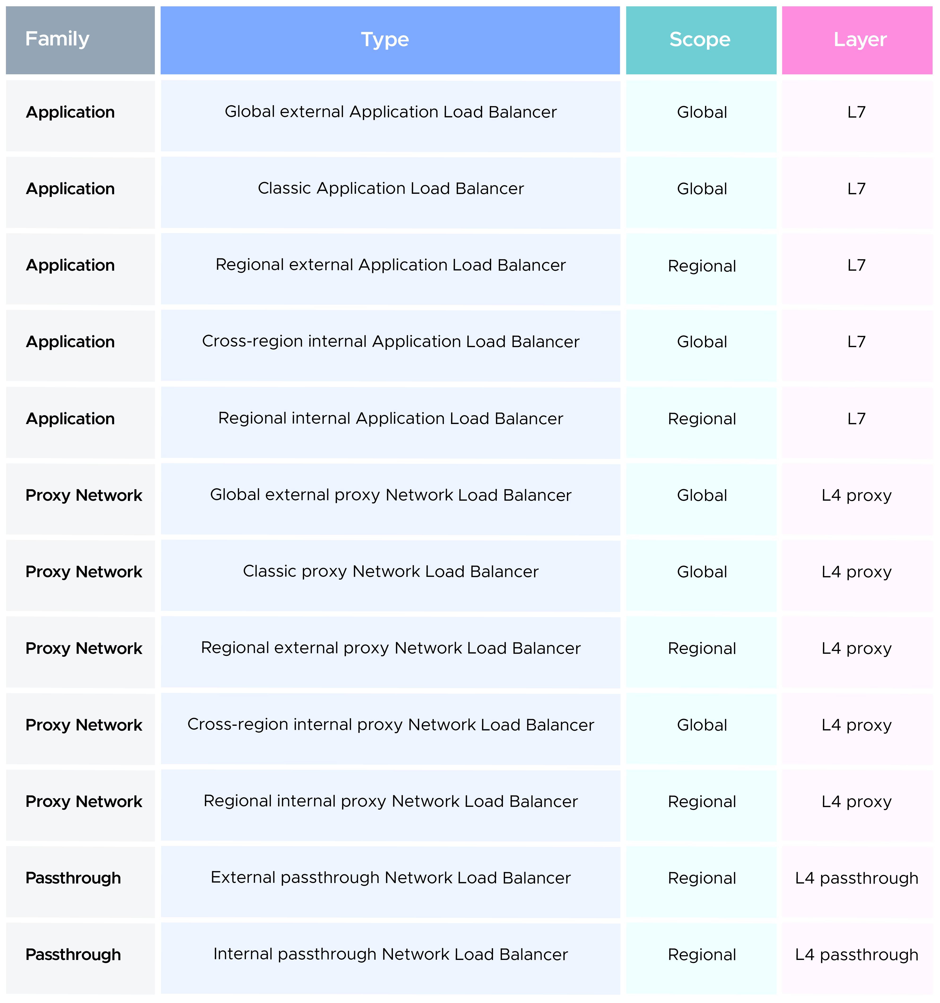
A classifier requires a marginally finer vocabulary than twelve. The classic proxy network load balancer exists in TCP and SSL variants that are distinguishable at the API and behave differently, and the external passthrough load balancer retains a legacy target-pool form alongside the modern backend-service form. Counted separately, these yield fifteen distinct classification outcomes, which is the granularity required to express a finding such as a recommendation to migrate a target-pool load balancer onto a backend service. Classification itself requires no inference; four signals taken from the forwarding rule are sufficient.

Load balancing scheme. EXTERNAL, EXTERNAL_MANAGED, INTERNAL, INTERNAL_MANAGED or INTERNAL_SELF_MANAGED. This separates internal from external and, within external, the classic generation from the modern one.

Scope. A forwarding rule carrying a region is regional; one without a region is global. Scope is also the indicator for the cross-region internal types, which Google Cloud models as global forwarding rules.

Target collection. The resource type the rule references: target HTTP proxies, target HTTPS proxies, target TCP proxies, target SSL proxies, target pools or target instances. This separates Application from Proxy Network, and TCP from SSL.

Structural signal. A rule carrying a backend service and no target is a passthrough load balancer, internal or external according to its scheme.

Three further target types are excluded for console parity: service attachments (Private Service Connect), target VPN gateways (Cloud VPN) and target gRPC proxies (Cloud Service Mesh). A fourth, target instances, constitutes protocol forwarding rather than load balancing and is reported under that designation rather than discarded, since it consumes an IP address and incurs charges.

Configuration attributes absent from billing data

On completion of the traversal, a single inventory row can carry sixty to seventy attributes for one load balancer, none of which appear in billing data. They fall into four groups.

Frontend. Forwarding rule count and names; IP addresses and address family; port ranges and exposed port count; network tier; network and subnetwork; global access on internal load balancers; all-ports configuration; source IP range restrictions; and the Private Service Connect connection identifier and status where applicable.

Security posture. Attached certificates and whether they are Google-managed or self-managed; days remaining before expiry; the applicable SSL policy and the minimum TLS version it enforces; whether an HTTP frontend has an HTTPS redirect configured; whether a Cloud Armor policy is attached; whether Identity-Aware Proxy is enabled; and the QUIC override setting.

Backend posture. Backend count and types (instance groups, zonal and regional network endpoint groups, serverless NEGs, internet NEGs and backend buckets); instance counts within those groups; attached health checks and the live health of each backend group at collection time; session affinity mode; connection draining timeout; balancing mode and capacity scaler per backend; outlier detection and circuit breaker configuration; and request logging status and sample rate.

Governance. Labels, descriptions, creation timestamps, and the set of other load balancers referencing the same backend services. The last of these is not derivable from any single resource and frequently indicates that separate teams have built independent frontends onto one application.

Most of these attributes are boolean or categorical, which is what makes them actionable. Billing data can establish that Cloud CDN incurred no charge during a period. Only configuration establishes whether that is because no cacheable content exists, or because the feature was never enabled.

Metric collection through Cloud Monitoring

Configuration establishes capability. Cloud Monitoring establishes behaviour across the selected window, typically the preceding thirty days.

Google Cloud does not publish a single set of load balancing metrics. It publishes seven, one per monitored resource family, and the applicable family follows directly from the type determined at classification.

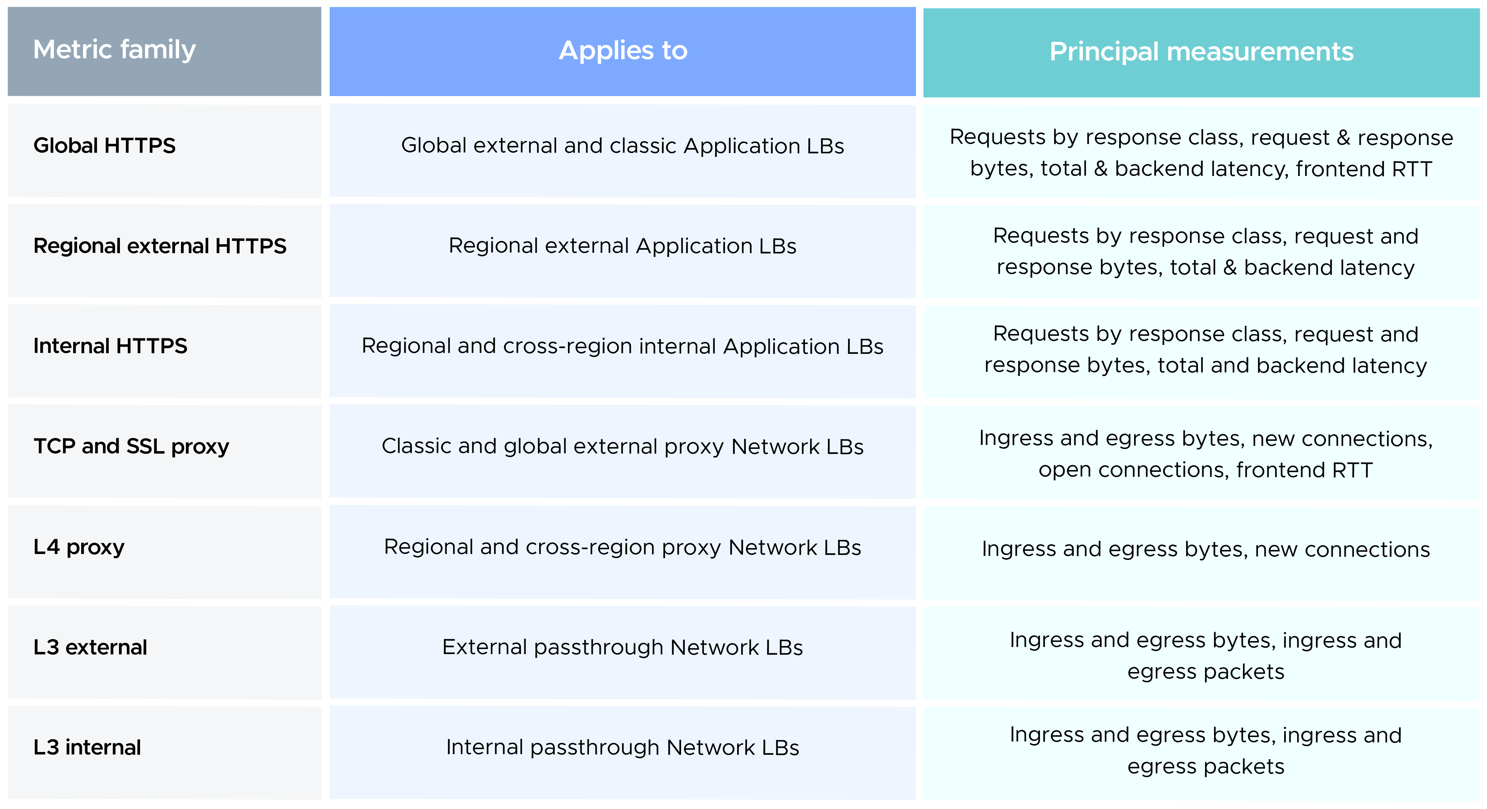
A query issued against the wrong family returns an empty result indistinguishable from a load balancer carrying no traffic. This is the most common origin of an incorrect idle-resource finding.

Identity resolution. Each family identifies the load balancer a series belongs to through a different resource label. Application load balancer metrics use the URL map name, proxy network load balancer metrics the forwarding rule name, and passthrough metrics the load balancer name. Certain internal Application load balancer resources report identity with a prefix consisting of a resource kind and a project number, rather than the bare name used by every other family. Both forms must be accommodated in the query, since the form a given project emits cannot be determined in advance.

Alignment. Counter metrics such as request and byte counts are summed across the window to produce a total. Latency and round-trip time are distributions and are aligned at the 95th percentile, since a mean value does not characterise the tail that determines user experience. Gauge metrics such as open connections are averaged.

Query construction and cost control

A single unfiltered query per metric per project is the lower-call-count approach, and also the one that routinely encounters Cloud Monitoring's own query-cost timeout on any project with sufficient load balancer count or traffic volume, because that cost is a function of series cardinality rather than window length. A query filtered to one load balancer's own identity remains inexpensive across a full thirty-day window, whereas the unfiltered equivalent can fail across a forty-eight-hour window. A larger number of narrow queries is therefore preferable, subject to a concurrency limit so that request volume does not itself create the load condition being avoided. Where a query does exceed the cost timeout, an unmodified retry cannot succeed; the documented remedy is to reduce the interval, which in practice means bisecting the window and querying each half.

Metric coverage as a reported attribute

Each row carries an explicit coverage state: Full, Partial, None, Timeout, Error, or Not applicable. The state is necessary because a zero carries two distinct meanings. A measured zero indicates that the load balancer served no traffic and is a deletion candidate. An unread zero indicates that the query failed, and acting on it would remove a resource carrying production traffic. An inventory that does not distinguish the two cannot safely be automated against.

Cost derivation from configuration and metrics

With configuration and metric data available, cost becomes a derivation rather than a lookup. Google Cloud load balancing charges resolve into three billing shapes.

External load balancers: forwarding rules and data processed

Every external forwarding rule is billed hourly irrespective of traffic. The first five in simultaneous use fall under a base hourly rate, and each additional rule is billed at a separate rate. A per-region charge then applies to each GiB of inbound and outbound data processed, and that volume is taken directly from the ingress and egress counters collected from Monitoring. Configuration supplies the rule count, metrics supply the volume, and the rate table supplies the price. No component is estimated.

One approximation should be disclosed on the row itself. Google Cloud applies the five-rule tier per project across all forwarding rules, not per load balancer. Pricing each load balancer against its own rule count therefore overstates the total marginally in any project containing several multi-rule load balancers.

Internal load balancers: proxy instances and data processed

This shape is the more frequently misapplied of the two, because an internal load balancer does not bill for forwarding rules and there is consequently no rule count to apply. The charge comprises the managed proxy fleet Google Cloud operates on the customer's behalf, billed per proxy instance per hour, together with a per-region charge for each GiB of data processed. The data-processed component is direct: internal load balancers do not publish separate inbound and outbound traffic, they publish ingress and egress bytes, which are summed into a single data-processed figure and multiplied by the regional rate.

The proxy-instance component must be derived, since the number of proxies in operation is not exposed in the Compute Engine API. Throughput is exposed, and the proxy fleet scales with throughput, so the count is reconstructed from bandwidth in four steps.

1. Sum ingress and egress bytes across the measurement window to obtain total bytes processed.
2. Divide by the window width in seconds to obtain sustained throughput in bytes per second. A thirty-day window is 2,592,000 seconds.
3. Divide that throughput by the volume a single managed proxy is taken to sustain, approximately 18 MiB per second, or slightly above 150 megabits.
4. Round up to the next whole instance, since proxies are not allocated fractionally.

As a worked example, an internal Application Load Balancer processing 230 TiB over thirty days sustains approximately 93 MiB per second. Divided by 18 and rounded up, this yields six proxy instances operating for 730 hours, to which the per-proxy-hour rate applies. A low-volume internal load balancer processing a few GiB per month resolves to one instance, the effective floor, and that single proxy-hour charge is the reason an idle internal load balancer is never free of charge.

Two qualifications apply. The figure of 18 MiB per second is a throughput assumption rather than a published constant, and is the only modelled value in the calculation. Because the derivation depends on measured traffic, it is valid only where metrics were successfully collected; an internal load balancer whose coverage state is Timeout has no derivable proxy count, and substituting one would be less defensible than disclosing the gap.

Smart Recommendations & Best Practices

Configuration, metrics and cost individually produce observations. In combination they produce recommendations, and the Well-Architected pillars provide a suitable classification framework.

Better Cost Management

This pillar is where the gap in billing data is most directly recovered.

• No utilisation in the reporting period. Forwarding rules are billed hourly regardless of traffic, so an idle load balancer represents a recurring charge with no offsetting value. This is the highest-value finding in the set and the most consequential to issue incorrectly, which is why it is gated.
• Forwarding rule count above the billed bundle. Only the first five rules in simultaneous use fall under the base charge. Consolidating frontends where protocol and address family permit removes the surcharge.
• Cloud CDN disabled on cacheable backends. Requests reaching the origin are charged twice, once as load balancer data processed and once as origin egress.
• Backend drained to capacity scaler zero. The backend receives no traffic while its instances continue to run and to bill. Either capacity is restored or the backend is removed.
• Premium Tier on a regional external load balancer. Where clients are co-located regionally and global anycast is not required, Standard Tier egress is materially less expensive, subject to validation of the latency requirement.
• Self-managed certificates. Google-managed certificates are provisioned and renewed automatically at no additional charge, removing both renewal effort and a class of expiry-related outage.
• Load balancer with no backends attached. The resource cannot serve traffic while its forwarding rules remain billable.
• Private Service Connect endpoint not in an accepted state. The endpoint holds an IP address and a forwarding rule without carrying traffic.

Improve Reliability. No health check attached. Backends reporting unhealthy at collection time. Server error rates above the threshold. A single backend behind a public frontend. Absent connection draining, under which deployments discard in-flight requests, and session affinity configured without draining, which amplifies the same condition. Absent outlier detection, under which a failing backend continues to receive traffic.

Increase Security. Plaintext HTTP with no redirect to HTTPS. Certificates expired or expiring within a week. A TLS frontend with no resolvable certificate. A TLS floor of 1.0 or 1.1. No Cloud Armor policy on an internet-facing frontend. No Identity-Aware Proxy where the workload is otherwise unauthenticated. An all-ports forwarding rule, or a passthrough load balancer without source IP restriction. A classic-generation type where a modern equivalent exists.

Performance. Total or backend latency above threshold at the 95th percentile, reported separately so that a slow application can be distinguished from a slow path to it. Elevated client round-trip time. Standard Tier where latency is material. Instance-group-only backends where network endpoint groups would route more directly. A capacity scaler below 1.0 constraining throughput.

Operational excellence and sustainability. Request logging disabled, or sampled below 1.0 on a load balancer of sufficiently low volume that full logging is inexpensive. Absent labels and descriptions, which render an idle load balancer unattributable and therefore undeletable. Legacy target pools. Configuration unmodified over an extended period. Monitoring data that could not be collected, reported as a finding rather than suppressed. Under sustainability: idle infrastructure, origin-only serving, duplicated frontends, and a global footprint provisioned for traffic that is entirely regional.

Constraints on recommendation validity

Utilisation findings are gated on coverage. Every traffic, latency and error-rate rule is suppressed unless the coverage state is Full or Partial. Where Monitoring could not be read, a zero request count denotes unknown rather than idle. Issuing a deletion recommendation on the basis of a failed query is the single error in this process capable of causing an outage, and the gate exists to prevent it.

The idle test is type-aware. Internal load balancers do not publish inbound and outbound traffic, only data processed. An idle test evaluated against inbound and outbound volumes would classify every internal load balancer in the estate as unused, and a report recommending the deletion of a hundred functioning resources will not be acted upon.

Each finding should additionally carry the documentation reference from which it derives. This is not presentational. The standard first response to any recommendation is a request for its basis, and an inline citation resolves that request without escalation.

Conclusion

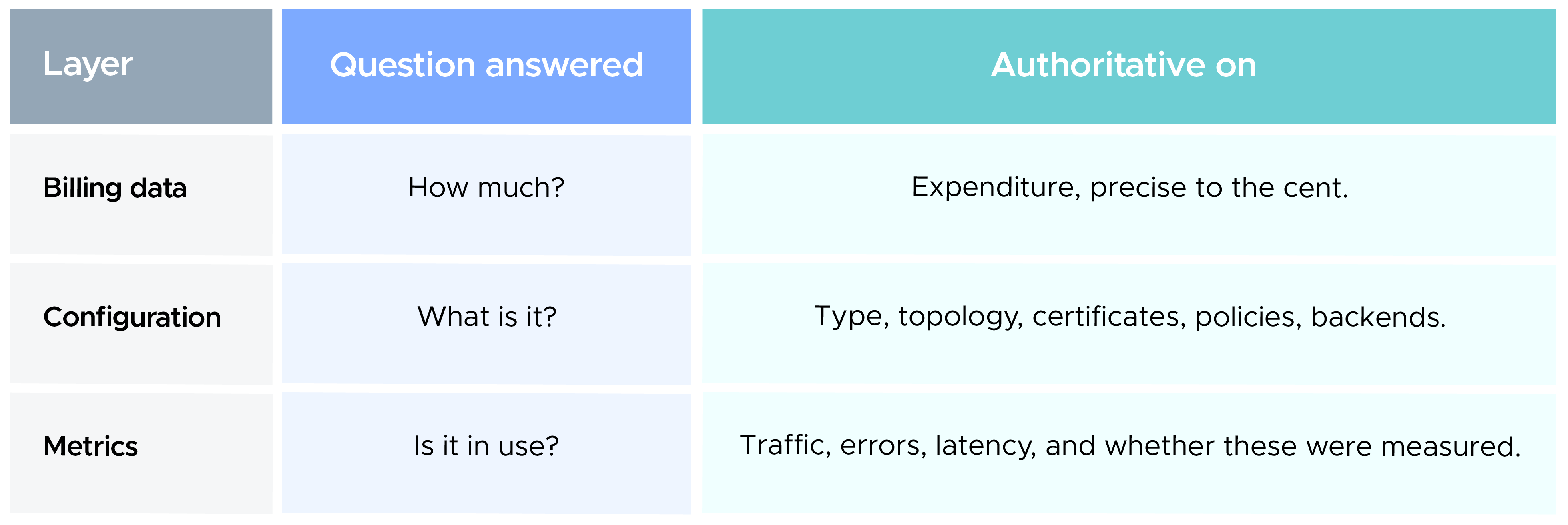
Billing data quantifies expenditure and is authoritative on nothing further. Configuration establishes what a resource is, what it permits and what protects it. Metrics establish whether it is in use and whether that determination rests on a measurement or on an absence of data. Only the three layers in combination support a remediation decision, which is the output the exercise exists to produce. A read-only service account, four APIs and a graph traversal represent a modest implementation cost for the distance between a figure that is accurate and a figure that is actionable.

A cost report is only as defensible as its weakest inference. Every figure produced by this process is either measured, derived from a stated model, or disclosed as unavailable.